ICGS: Unsupervised Single-Cell Population Identification
Iterative Clustering and Guide-gene Selection (ICGS) version 2.0
ICGS2 is a new computational approach that can resolve rare and transitional populations in single-cell (scRNA-Seq) datasets. A preprint manuscript describing ICGS2 will be available soon on bioRxiv and a video tutorial on ICGS2 and cellHarmony is available here. Sample data for analysis can be found in the latest version of AltAnalyze (version >=2.1.2) in the DemoData/ICGS folder along with instructions. ICGS is a multi-step algorithm in AltAnalyze which applies intra-gene correlation and hybrid clustering to uniquely resolve novel transcriptionally coherent cell populations.
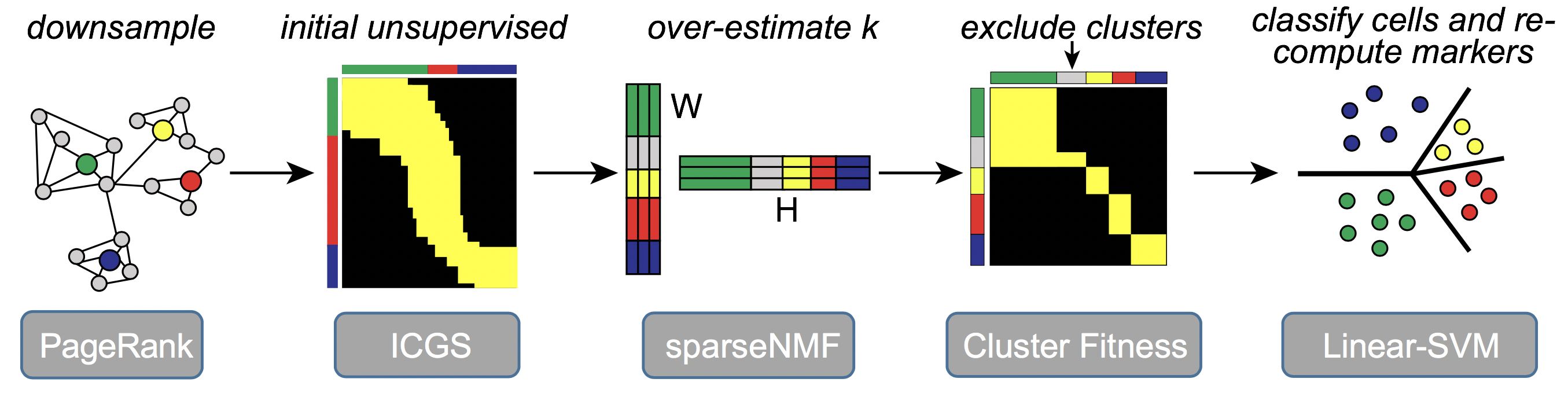
The software ICGS2 has been developed as part of an open-source python toolkit, AltAnalyze, with a complete documentation of its use, algorithms and optional user-defined parameters (https://altanalyze.readthedocs.io/en/latest/). ICGS2 identifies cell clusters through a five-step process: 1) PageRank-Down-sampling (optional), 2) feature selection-ICGS2, 3) dimension reduction and clustering (sparse-NMF), 4) cluster refinement (MarkerFinder algorithm), and 5) cluster re-assignments (SVM).
 .
.
ICGS2 performs the following steps: 1. Performs down-sampling using PageRank to reduce the number of cells to be analyzed by the downstream tools. For extremely large datasets (cells >25,000), Louvain clustering at minimum resolution is performed additionally to reduce the samples. This step is optional to improve speed of the approach. 2. Performs feature selection using the original version of ICGS to identify highly correlation gene modules. Generates several outputs including Guide1, Guide2 and Guide3 results. 3. Guide3 ICGS file is used to estimate k and supplied to SNMF. SNMF factorizes the matrix (Guide3 file) to generate a basis matrix W (dimensions, number of cells x number of k’s). 4. The W matrix generated is binarized i.e. 1 when the cell has the largest contribution to the rank and 0 otherwise. 5. Each rank (cell cluster) in the W binarized matrix is considered as a reference and MarkerFinder is performed to identify the top genes associated with these ranks. 6. Cluster fitness is performed to exclude cell clusters that do not have sufficient genes associated with it based on the fitness criteria. 7. Linear SVM is performed to to re-assign cells to cell clusters that satisfied the fitness criteria. Additionally, when down-sampling is performed, Linear SVM is used to assign the remaining cells to the identified clusters.
Running ICGS2 through the AltAnalyze Graphical Interface First, download either latest pre-compiled version of AltAnalyze from http://www.altanalyze.org or source code versions from PyPI (pip install AltAnalyze). Install the appropriate species gene database when prompted. ICGS should be run with HOPACH clustering. The R library HOPACH will be automatically installed by AltAnalyze (except when the user does not have administrative privileges) when R is already installed on the computer (https://cran.r-project.org/). Users can supply diverse input file formats including a normalized counts text files, 10x Genomics (h5 or mtx), FASTQ or BAM files. For FASTQ and BAM file inputs, each file must currently correspond to an individual cell library. An example video tutorial for processing these data is found here.
Steps
- Open AltAnalyze and proceed to the main menu. AltAnalyze can be run from the pre-compiled binary file (double-click) or from the command-line when installed through PyPI (type AltAnalyze in the terminal). Select your species and platform for analysis. For 10x Genomics h5 or mtx inputs, select 10X Genomics aligned from the Select Platform menu.
- In the following Select Analysis Methods menu, select the top menu option to process raw data (Process Chromium Matrix/Process RNA-seq reads) or a pre-processed normalized expression matrix (Process Expression file). Note, if beginning with a text file containing counts (csv, tsv, or text), this file can be column normalized for total counts per cell using the AltAnalyze script import_scripts/CountsNormalize.py as: python CountsNormalize.py --i "/users/data/wt_counts.txt".
- In the subsequent menu, select the input file (text, h5, mtx) as prompted or directory of input BAM or FASTQ files, along with the directory in which you want the analysis results saved to. After selecting continue, the program my lag for a moment, as it copies necessary input files to the output directory.
- In the following two menus, the user can accept the default options or customize. These impact the stringency of post-ICGS2 analyses (optional), including pathway analyses and differential expression analyses comparing adjacent cell populations.
- In the Assign files to a Group Annotation menu, select the option Run de novo cluster prediction (ICGS) to discover groups.
- In the ICGS Main Menu, accept the default options (recommended) or modify as desired. The software begins with a low correlation cutoff and dynamically adjusts as needed (increases when initial correlated genes are >5000). Options that most significantly impact downstream cluster prediction are:
- Select the column clustering metric (cosine and euclidean recommended)
- (optional) Eliminate cell cycle effects (select conservative to exclude)
- (optional) number of user-defined ICGS cluster (k). By default, the program will determine automatically.
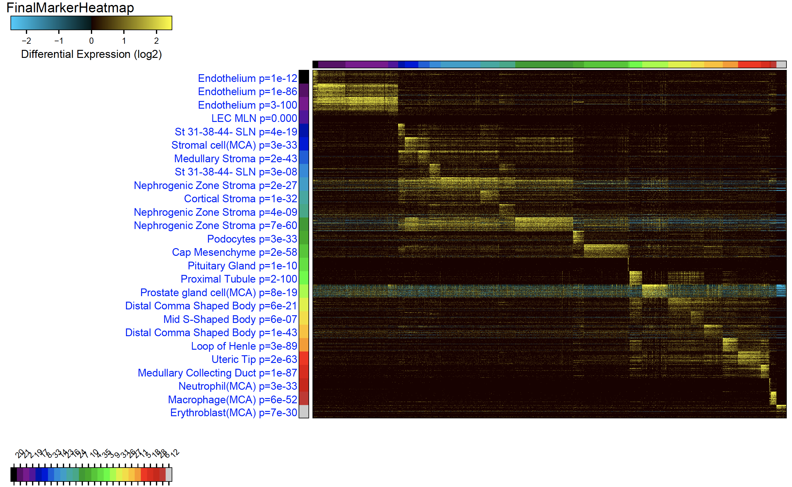
- Once run, the final ICGS clustering results will be displayed. The final results will can be found in the folder ICGS-NMF and secondary results in the folder ICGS. These include cell to cluster notations, UMAP plots, marker gene heatmaps and cluster marker genes.
Cell-Type Predictions and Heatmap Output of ICGS2
Running ICGS2 through the AltAnalyze Command Install AltAnalyze through PyPI:
pip install altanalyze
Install the appropriate species database:
AltAnalyze --species Hs --update Official --version EnsMart72 --additional all
Run ICGS:
AltAnalyze --runICGS yes --platform RNASeq --species Hs --removeOutliers yes --excludeCellCycle conservative --ChromiumSparseMatrix tests/demo_data/10X/input/filter_matrix.h5 --expname cancer --output /tests/demo_data/FASTQ/output/ --downsample 2500
Additional examples Can be found here.
Core ICGS algorithm
ICGS includes multiple options for filtering the expression data based on normalized gene values (e.g., TPM, FPKM), fold change, correlation thresholds for identifying the most coherent gene sets, clustering algorithms (e.g., HOPACH) and optional supervised clustering options using custom or established gene-sets, pathways or Ontology terms. Gene clusters containing multiple cell-cycle-annotated genes can be optionally excluded from the software graphical user interface. Results for each stage of clustering are stored and presented back to the user as a heatmap and HOPACH cluster sample. For the five separate heatmap results generated at each stage in the analysis, the user can select one of these for further analysis as pairwise group comparison between all possible HOPACH clusters using the default AltAnalyze gene and alternative splicing analysis workflows. While the ICGS analysis is being run, the software performs the following steps:
Step 1 - Pioneering Round Analysis
In this first round of analysis, all input gene expression values are analyzed and subsequently filtered to exclude low expression, low-variance transcript and weakly-correlated genes. For single-cell libraries an already normalized gene expression matrix (RPKM, FPKM or TPM) or aligned read counts files can be used as input for this workflow. For aligned read counts, these can be provided as TopHat-produced junction.bed, BedTools exon.bed or TCGA junction expression files, among others. Using the graphical user interface, ICGS can be parameterized to restrict the analysis to protein-coding genes, exclude genes with a maximum expression value (RPKM, FPKM or TPM) and a minimum expression difference (fold change) between the lowest and highest expressing libraries for each gene (number of samples differing must also be indicated by the user). A correlation threshold must also be provided to indicate the minimum relative similarity required to report correlated genes for downstream analyses. Based on the supplied correlation cutoff, ICGS retains genes (initial guide genes) correlated to at least 5 others (protocluster). A secondary filter is to exclude protoclusters in which a single outlier cell for the initial guide gene is driving the protocuster correlations. To this end, at least 50% of the protocluster genes must remain correlated to the initial guide gene after temporary exclusion of the most highly expressed cell for the initial guide gene. Using the HOPACH clustering algorithm, through an optional connection to R and bioconductor, “Pioneering Round” clustering results are obtained for all remaining filtered protocluster genes (Figure 1, left).
Step 2 – Reduce Cluster Complexity
As many gene clusters are produced following the initial round of HOPACH, each with different sizes, the software performs a pruning step to produce clusters of more similar number of genes (3 to 50 genes). This is accomplished by first identifying the genes in each cluster that are correlated to the most members in that cluster (greater than the input Pearson correlation cutoff). This step further improves cluster definitions by removing genes and clusters with lower overall intra-correlation. What is left are a smaller set of genes, highly correlated to each other and largely distinct from other HOPACH clusters. These genes are again clustered with HOPACH to produce more coherent signatures.
Step 3 –Selection of Guide Genes Round 1
Following HOPACH clustering, the algorithm selects the top intra-correlated gene(s) for each gene cluster (correlated to the most members in that cluster with the provided Pearson correlation cutoff), and any gene encoding transcription factors present in that cluster (UniProt or Gene Ontology defined) as guide-genes for the following round of clustering. At this stage, gene clusters and guides with 2 or more Gene-Ontology-defined cell-cycle genes will be optionally excluded. All genes from the initially filtered expression dataset are correlated to these guide genes (positive correlations only) using the user provided cutoff (maximum of 140 correlated genes per guide gene), to obtain guide correlated gene sets that are clustered again with HOPACH.
Step 4 – Selection of Guide Genes Round 2
Following HOPACH of the guide-correlated genes, additional genes will be brought into the analysis that contain new potential guide genes. To discover these, the resulting HOPACH clustered genes from Step 3 are subjected to the protocol in Step 3 to select new distinct guide genes. As before, HOPACH clustering is run and the results stored.
Step 5 – Final Clustering Using All Guide Genes
Combining the guide genes identified in Steps 3 and 4, Step 3 is repeated once again and a final clustered heatmap is produced. These clustered results are presented with all other in the AltAnalyze graphical user interface. The user can choose to quit the analysis and work with the produced clustered sets or select specific heatmap and cell-clustering results for downstream comparison analyses in AltAnalyze.
Downstream Comparison Analyses in AltAnalyze (Optional)
In the graphical user interface, the user is presented with the option of selecting any of the resulting cluster outputs from ICGS for further AltAnalyze-based comparison analyses between the defined HOPACH cell cluster groups. These analyses include all pairwise group comparisons using the selected statistical test (e.g., moderated t-tests, Benjamini-Hochberg adjustment), pathway analysis in GO-Elite, PCA, MarkerFinder, pathway visualization and splicing analyses, when exon or junction data is available.
In addition to these AltAnalyze workflows, further analysis of the ICGS clusters can be performed using the built-in hierarchical clustering tool using the advanced options available. These advanced options include the ability to interactively display enriched pathways, ontologies or other gene sets to the left of the heatmap, run Monocle R library, obtain all correlated genes to a manually supplied guide gene or available gene sets. For the current analysis, genes associated with Neutropenia or MDS/AML were input as manual guide genes to obtain correlated gene sets using a supplied Pearson correlation cutoff of 0.4. Step-by-step tutorials and videos illustrating this workflow are available from the AltAnalyze website.